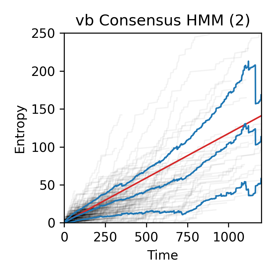
Plot Entropy

Here’s a full script that you can use to plot the entropy of your trajectories. Note that you must have a model first (otherwise you cannot know the probabilities). In general, you should save this as a .py file, and use the Scripts >> Run Scripts menu option to run that file. You can edit it as you go if you want to change something, and then re-run it. Note that it use’s the current activate model for the calculation.

Save the code below in a file as plot_entropy.py

import numpy as np
import matplotlib.pyplot as plt

def calc_entropy_expected(A,pi):
    Hxavg = -np.sum(pi[:,None]*A*np.log(A))
    H_expected = Hxavg
    return H_expected

fig,ax = plt.subplots(1,figsize=(3,3),dpi=300)

m = maven.modeler.model
nt = maven.data.nt
nk = m.nstates
kb = 1.

Tmc = m.tmatrix
A = Tmc.copy()
for i in range(A.shape[0]):
    A[i] /= A[i].sum()

# pi = m.frac
# pi /= pi.sum()

w,v = np.linalg.eig(A.T)
ind = np.where(w==w.max())[0][0]
ss = v[:,ind]
ss /= ss.sum()
pi = ss

vits = m.chain
nmol,nt = vits.shape
ss = np.zeros((nmol,nt)) + np.nan
pre = maven.data.pre_list
post = maven.data.post_list
dp = post-pre

for nmoli in range(nmol):
    v = vits[nmoli]
    if dp[nmoli] > 1:
        ri = m.r[nmoli].copy()

        # ## use viterbi instead of the full chain
        # v = v[pre[nmoli]:post[nmoli]].copy()
        # pij = pi[v[0]]*np.concatenate(([1.],np.exp(np.cumsum(np.log(A[v[:-1],v[1:]])))))
        # sij = -kb*np.log(pij)

        ## use full gamma treatment
        pij = np.zeros((dp[nmoli]))
        pij[0] = np.log(np.sum(pi*ri[pre[nmoli]+0]))
        for t in range(1,dp[nmoli]):
            pij[t] = np.log(np.sum(A*(ri[pre[nmoli]+t-1][:,None]*ri[pre[nmoli]+t][None,:])))
        sij = -kb*(np.cumsum(pij))
        sij[np.isinf(sij)] = np.log(np.finfo(np.float64).max)
        sij[np.bitwise_not(np.isfinite(sij))] = np.nanmax(sij[np.isfinite(sij)])
        ss[nmoli,pre[nmoli]:post[nmoli]] = sij

dt = maven.prefs['plot.time_dt']
x = np.arange(nt) 

for nmoli in range(nmol):
    ax.plot(x*dt,ss[nmoli],color='k',lw=1,alpha=.05,zorder=1)


sexp = calc_entropy_expected(A,pi)
theory = x*sexp-kb*np.sum(pi*np.log(pi))
ax.plot(x*dt,theory,color='tab:red',ls='-',lw=1.2,zorder=1)
desc = m.description()
desc = desc.split('] ')[1]
desc = ''.join(desc.split(' -')[:-1])

low,med,high = np.nanpercentile(ss,[2.5,50.,97.5],0)
std = np.nanstd(ss,axis=0)
mean = np.nanmean(ss,axis=0)
ax.plot(x*dt,mean-std,color="tab:blue",label ='%s'%(desc),ls='-',lw=1.2,zorder=2)
ax.plot(x*dt,mean,color="tab:blue",label ='%s'%(desc),ls='-',lw=1.2,zorder=2)
ax.plot(x*dt,mean+std,color="tab:blue",label ='%s'%(desc),ls='-',lw=1.2,zorder=2)


#### order the traces. This destroys the matching w the HMM viterbis so... annoying
# order = np.nanmax(ss,axis=1)
# print(ss.shape,order.shape)
# order[np.isnan(order)] = 0.
# order = np.argsort(order)[::-1]
# print(order)
# maven.data.order(order)
# maven.emit_data_update()


ax.set_ylim(0,np.log(np.finfo(np.float64).max))
ax.set_ylabel('Entropy')
ax.set_xlabel('Time')
ax.set_title(desc)
ax.set_xlim(0,x.max()*dt)
fig.tight_layout()
plt.show()